ASCII Art

I've been looking at ASCII art recently - at least in the context of
converting images into ASCII-rendered versions of the original. This has
resulted in a few simple projects including one where I rendered a webcam
video feed as ASCII in a terminal. One of the challenges I faced in that
project was finding the correct size of the font to get reasonable results; a
standard 80 x 24 terminal left a lot to be desired in terms of the final text
rendering of a video frame. It was easy enough to simply resize the
font/terminal to get what I wanted but it wasn't a very elegant solution and
didn't translate very well to other projects (where the render target was not
a terminal, for example). 

To address that limitation I ended up writing a dynamic font 'renderer'[1] -
this post describes some aspects of that project.

The interesting parts (to me) include the font rendering/scaling,
the tiling of the image parts, and the interesting combinations of rendering.

Dealing With Fonts

This was mainly familiarizing myself with the FreeType font library and how
to load and render fonts in memory. I could have just taken one of the many
already existing ASCII-to-grayscale mappings but I wanted the ability to
provide a few additional features that required more than that (e.g. custom 
character sets and non-fixed-width fonts).

So, rather than use an fixed set of characters I dynamically compute
the average brightness of a particular character set (for a given font) and
use that to select glyphs to replace image pixels.

In addition to which font and glyphs to use I also dynamically scale
the glyphs used based on properties of each region of an image. The FreeType 
font library supports this directly allowing me to render a glyph at whatever
size I specify; I can then 'copy' those pixels directly to the translated image.

Image Tiling

I used a windowing mechanism to select the size of the font to use. Given an
image, I subdivide the image into N rows and M columns and in each N,M cell
select a font size (more on how a size is selected later).

Then, within that cell, compute the properties of the region for each character
glyph and translate that source image region to an ASCII character that most
closely matches the average greyscale value of that region.

This nested tiling approach allows for selecting font sizes in any number of
ways. For example, selecting a random font size within each N,M cell of the
image results in the following.

Zooming in on a section of that images highlights a few things about this
approach:

there is flexibility of rendering each region in isolation
clipping at the edges of regions will start to produce artifacts in the 
output image due to discontinuities between the glyphs
as you approach a glyph size of 1x1 you approach a pixel-level copy of
the original image region

Of course, just like the impetus for this project, there is something left to
be desired about the resolution of the final image. Select a size too large
and there is loss of detail; too small and the 'ascii' effect is dimished. 

So I started experimenting with ways to quantify the amount of resolution
in a section of the image and how to translate that to font size.

Rendering

Finding the right way to encode resolution turned out to be a bit of a rabbit
hole for me. I started with the idea of using the entropy of each window but
broadened my search to frequency- and thresholding-based techniques.

RMS

A basic root mean square approach captured some of the contrast in the image
but it wasn't sufficient for what I wanted.

Frequency Domain

After a bit of research I came across a paper "Contrast in Complex Images" by 
Eli Peli which discussed how the human eye perceives contrast and various ways 
to compute that spatially across an image. It fit nicely into the notion of a 
subdivided image and provided an equation to compute sub-cell contrast based on 
high-frequency components in an image.

Essentially this consists of taking the DFT of an image, running that through
a high-pass filter, and computing the inverse DFT of the filtered content.
This is closely related to edge detection but maintains more high-frequency
information (as you can see in the examples below).

This worked well for some images, but the residual information created some 
noise for certain image types. Consider the two images: kitten and wave.

The contrast is easier to identify in the kitten but the wave is a bit more
challenging.

Thresholding

Finally, I ended up using a tunable threshold technique where I convert the
image to B/W based on some threshold brightness and use the proximity to this
threshold value as an indicator of the amount of contrast in each window. This
ultimately ended up working fairly well for the effect I was looking for
preserving much of the data of the frequency-based approach but without the
residual noise.

[1] I say renderer but I use libfreetype to do all the heavy lifting of
pixel-level character rendering.

Tiny Spell Checker (Part II)

In the previous post I introduced the tiny spell checker challenge and some of the solutions our team discussed. In this post I'll go into a bit more detail about the solution I put forward, how well it performed, and some limitations of the approach.

I combined the use of a bloom filter with additional validation using n-grams.

Bloom Filter

The bloom filter is a well-known data structure for checking the existence of an element in a set. The bloom filter provides good space efficiency at the cost of a probabilistic result. In other words, you can ask whether an item exists within a set and get one of two answers: no or probably. You can control how often probably is returned for an item that is not in the set through a few parameters: the number of items in the filter, the number of bits in the filter, and the number of hash functions used to compute the bit indices. 

In my case, the input size was fixed (the number of words in the dictionary) so I could control the number of bits and the number of hashes. Since this challenge was primarily about size I fixed the number of hashes and experimented with a bit count that would fit within the challenge constraints. 

That left me with a calculated probability of returning a false positive somewhere around 1 in 3. We will see how this ultimately impacts the performance of the spell checker below. However, there was still a bit of space remaining to attempt to reduce the number of false positives so I looked to using something else I was exploring in parallel: n-grams.

N-gram Validation

I spent a significant amount of time while exploring the solution thinking about compression. How could I compress the 6.6M to something even close to the 256K size limit for the challenge (zip gets close to 1.7M, for example). As part of that I looked into n-gram substitution - specifically, could I take advantage of known suffixes or prefixes to reduce the amount that needs to otherwise be compressed. 

This ultimately didn't pan out as I ended up needing to store more in metadata to decode the table than the size reduction of the approach. However, one of the challenges with bloom filters is false positives, especially when the table size is constrained and there are many inputs. So when I pivoted to using a bloom filter I returned to the n-gram approach as as a secondary validation mechanism. 

For each of the words in the dictionary I extracted each n-gram and added it to a set. Checking for a valid word then consisted of extracting each n-gram of the input word and verifying it was part of the set.

Much like the bloom filter this has the property of no false negatives (i.e. any n-gram not in the set must be from a misspelled word) with the potential for false positives (i.e. can construct a word from the n-grams set that is not a valid word from the original dictionary). 

For the 6.6M dictionary, the following table indicates the space necessary to encode all of the n-grams of a particular size. 

N	Size
2	1,766
3	33,892
4	330,872
5	1,459,024

To keep within the size constrains of the problem I could only use n-grams of size 2 or 3. I wanted the larger since this was for validation and I felt there would be higher false positive rate using the shorter n-gram size (although, to be fair, I did not measure this).

Building Metadata into the Executable

As I wanted an all-in-one solution, I serialized both the bloom filter and n-gram set to disk as a separate process before building the executable. 

I used a std::bitset for the bloom filter and made sure to set the size to something divisible by 8 so it was possible to serialize without accounting for padded bits. For the n-gram set I ended up using std::set< std::string > so serialization was just a matter of writing the 3-byte sequences out to file. The order in the set didn't matter so I could simply dump the values contiguously given I knew the n-gram size.

With both data sets serialized to disk I used the linker to generate object files out of the binary data so I could link them when building the final executable.

$ ld -r -b binary -o ngram_data.o ngram.bin

$ nm ngram_data.o 

0000000000008464 D _binary_ngram_bin_end

0000000000008464 A _binary_ngram_bin_size

0000000000000000 D _binary_ngram_bin_start

Limitations

Capitalization: To achieve some of the size results I had to make some concessions. For example, all string operations (hashing and n-gram) is performed on lower case strings. This completely removes any capitalization support in this application (a necessary feature for any serious spell checker). 

Speed: Because of the way the dictionary is packed, there is a large upfront cost (relative to the check itself) to load the information into usable data structures before a single word can be checked. I would have liked to have had something that could be searched directly from memory but opted for a more simplistic serialization approach instead.

Results

I computed the full dictionary (6.6M) for n-grams of size 3, hashed each of the 654K words for the bloom filter, and serialized and linked each of those into an executable that came in at 243K. 

In the worst test case (replacing 50% of the dictionary words with invalid words) the f-score was about 0.86 without using n-grams and closer to 0.88 with n-gram validation.

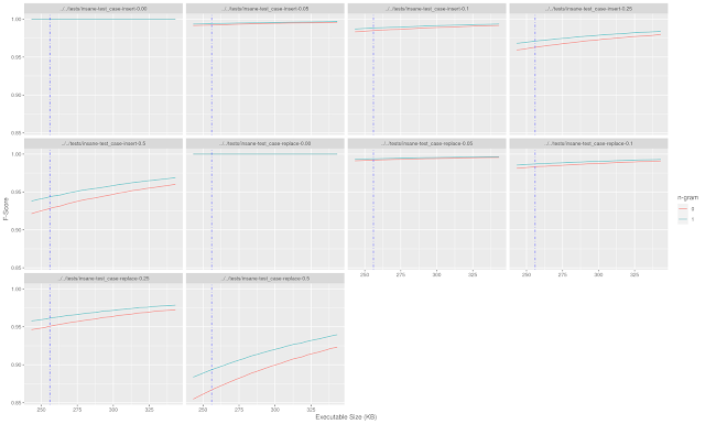
Looking back at the expected false positive rate of the bloom filter (roughly 1 in 3) this is the expected output. With a 654K input, 50% of which are replaced with invalid words, we would expect somewhere around 115K false positives which is consistent with an f-score near 0.85.

Adding in the n-gram effectively helps lower the probability of a false positive from 1 in 3 to just over 1 in 4. There is plenty of room here for optimizations such as fine-tuning the bloom filter to be closer to the size limit, pruning the n-gram list to the most frequent values to reduce size, and so on, but this was a decent start to thinking about the problem.

Tiny Spell Checker (part 1)

Inspired by a post I read about how designing a spell checker used to be a major software development effort[1] I designed a coding challenge of sorts for the teams I work with. We have these types of technical exchanges semi-regularly as a way to collaborate and explore technology problems; they also serve as a great team building exercise.         

I'd like to introduce the problem here and some of the solution space we considered. I plan on providing a bit more detail about my final solution in a future post. 

As an aside, we generally avoid making this competitive; it decreases participation and distracts from the main purpose of exploring the problem space and learning about others' approaches (which may be entirely non-technical).

Below are some of the topics we discussed during the showcase. The topics are primarily centered on various compresssion mechanisms (lossless and otherwise) as you might expect. However, there were additional conversations that considered a broader context. For example:

• translating to another language which had better compression properties 
• using phonetics (stenography)
• a literature survey of compression techniques
• trade-offs in time, space, and accuracy of each approach

It is those last two bullets that really highlight the benefit of these exchanges. 

It is one thing to be able to implement a decent compression algorithm; but learning how to consider the problem under extended or different constraints allows us to apply these ideas to the projects we are working on and generally makes us better developers.

Asymmetric Numeral Systems (ANS)

A set of entropy encoding methods that include probability distributions and finite state machines which combine to achieve performant compression. In particular, we discussed the table-based version of ANS (tANS).

Huffman Coding

Lossless compression technique that uses symbol frequencies (probability) to build a table for encoding symbols relative to their frequency: the more frequent a symbol the fewer the bits used to encode it.

Some additional discussion was the cost of using a well-known table or building it from the input dictionary and storing it in the encoded (compressed) output.

n-grams

Encoding common groups of letters into a single symbol/value. For example, encoding the sequence "ing" as a single value. 

This is very similar to Huffman but operating on n-grams instead of a single byte.

Rabin-Karp

Is an algorithm for searching for a string in a body of text. At a high level it leverages a hash to do approximate string matching and only does full string matching if there is an approximate match.

Trie

A data structure that encodes words in a prefix tree and indicates whether a particular word exists in the tree (i.e. is valid) when all letters follow a path in the tree and end at a word terminator node.

Bloom filter

A data structure that, given a hash function, can answer either: an element may be encoded in the set; or it is definitely not in the set. That is, there is the possibility for false positives but not false negatives when checking for existence of elements.

A nice property of this data structure is that it has known properties regarding the false positive rate given a size and hashing strategy used so it can be tuned to a specific accuracy given size constraints.

Affine Transformation

I've been working on a personal project for data presentation and exploration. It is very much a work in progress but as part of the development I've come across some interesting little technical problems to solve. I hope to eventually have a longer series of posts along the lines of 'building your own data tools;' however, until I find the time to give that the attention it needs, I plan on posting some smaller entries centered around these technical problems.

One of the early challenges I came across when plotting data was mapping the input values to the fixed amount of space I had on screen. For example, if I generate a window that is 600px wide I can only support a range of input values less than or equal to 600 (using a naive approach of each value in the range maps to a pixel on screen). Supporting an input range greater than 600 values requires some level of mapping between the input values and the available pixels on the screen. There are simple conversions for specific input ranges (e.g. when the range is close to a multiple of the number of pixels) but a more general solution is necessary to handle arbitrary input data sets.

The way I ended up solving this was to use an affine transformation to map the input domain to a fixed pixel range. This is how scales work in D3.js if you are familiar with that JavaScript library. For example, if my input values come from [-100, 100] but I need my output values to fall within [28,63] then applying this transformation would look something like the image below:

Notice that the minimum value in the input interval (-100) maps directly to the minimum value in the output interval (28). Values along the input interval are mapped to the output interval preserving the relative position within each. The equation to do this is:

\[ range_{x} = (domain_{x} - domain_{a}) * ((range_{b} - domain_{a}) / (domain_{b} - domain_{a})) + range_{a} \]

Where domain and range are defined by the intervals \([domain_{a}, domain_{b}]\) and \([range_{a},range_{b}]\), respectively. Neither the domain nor the range is required to have a 0 as one of the endpoints and the intervals can be either increasing or decreasing. This generality is helpful in a variety of contexts. For example:

Setting Borders

The viewport used to plot data may not always use all available pixels of the window; multi-plot windows or viewports that have a border are two examples. In the case where there is a border around the plot (allowing for labels and tick marks) that area should not be considered as part of the range of the viewport. Instead, a window with 600px width that uses 30px on either side for border should use a range of [30,570] - the equation above makes this easy.

Inverted Axis

In most window coordinate systems the origin is at the top left of the screen. That means increasing y-axis values (from the window perspective) are typically decreasing data set y-axis values. Using a negative range makes this translation simple. Consider a 600px window height: mapping a domain to the range [600,0] automatically handles the inverted axis problem.

Another way that this simplifies things is when there is a need to 'flip' the layout of a graph. For example, in the two images below the data is the same; the only difference is the range. Having the ability to easily manipulate target ranges for the input data allows me to cycle through multiple views of the same data without much work on the backend.

 

Visualizing Network Traversal

As part of an experiment I was doing related to network traversal I started to trying to visualize coverage of a network by a single visitor traveling through the nodes. The idea was to set a gradient between two colors and as a node was visited more times it would slowly take on a change in color over the gradient. If the goal was to visit each node N times, then the visualization would indicate current progress as a 'heat map' of the network according to the number of visits to each node.

The outputs were interesting in that controlling the traversal policy would change the distribution of color over the image. This is perhaps obvious given the experimental construct but still provided an alternate mechanism for 'measuring' the accuracy of the traversal. For example, if the goal is to cover the network as evenly as possible during the traversal, the kurtosis of a distribution then becomes a measure of how close one is to this goal.

To demonstration this I set up an NxN grid network and ran three example traversals over that grid. I captured the 'heat map' when the median of all the visit values for the nodes was at half of the target visits. The results are below.

Random Choice Walk:
At any node, a visitor will choose to move up, down, left, or right by random selection.

Backpressure Walk:

Uses a notion of backpressure to control the traversal. At each node, a visitor checks for the the least visited neighboring node and travels there.

Teleportation:
Not really a traversal, I just did it to see what it would look like. At each node, a visitor chooses a random node within the grid and jumps there directly.

Water Bleed Image Effect

Recently, I had the occasion to play with some features of the amazingly powerful ImageMagick image manipulation tool. After playing with several of the command-line tools and manipulations I decided to look into the API provided through the MagickWand C interface to ImageMagick. To explore some of the features available at this layer I'm attempting to develop a bleed effect on an image; similar to if you had dipped a picture in water and then hung it up to dry. I'm hoping that my free time permits and I can turn this into a small series of posts detailing how I refine this tool (if I can eventually call it that).

Perhaps in a later post I'll get into what the code looks like and a dialog of what each part does but for now I'll just put up some of the early results and learning points that I've encountered. Ultimately, I'll get the code up on github and follow along with that here.

I'm using two images for this exercise: one that contains a rainbow of colors to test and another to represent the effect on a more likely picture.

Initially, I looked at just 'dragging' each color down the image while increasing the normalization scale along the vertical to give a wash out effect further down the image. This represents how the water would continue to wash color away as it 'pulled' higher colors down the hanging image. This worked well for the rainbow version of the image:

That result has a good 'bleed' in that stronger colors last longer down the vertical. However, with the colors in the house image the washout was too aggressive and wiped out much of the original content.

If you ignore the washout, though, it is clear that the draw of colors down the image is visible (especially around the windows) meaning that reducing the washout might still produce a more realistic effect if enough of the original image could be preserved.

With that in mind, I added the ability to preserve a percentage of the original image while applying the effect. This allows a user to tune the washout per image to get just the right look. For example, too much reuse (20%) on the house and the washout effect has little impact:

But taking that down to 7.5% gets closer to what I am looking for:

There is still plenty for me to do such as handling the edges and water line better and further manipulating the washed image. For example, adding additional transforms to the result to get more seep/bleed on the washed colors. The image below shows a simple kernel convolution to add blur to the pencils, for example.

Derive formula to convert Fahrenheit to Celsius

I had been revisiting linear regression the other day and as part of that review I challenged myself to use regression to derive a well known formula without actually looking it up (the formula, that is).

The first example that came to my mind was the formula for converting temperature in Fahrenheit to Celsius. I wanted to see if I could derive that formula using two sample data sets and a simple linear regression. If the data was accurate enough, I should be able to derive the exact equation for converting between the two formats. In essence, I wanted to be able to come to the following:

C = (F - 32) * 5/9

Since I didn't have a data set with both types of observations available I was faced with a little 'chicken or the egg' situation. Seeing how this is just a fun little exercise I generated my own data introducing some artificial error to stand in for true observations.

After the 'observations' were available the regression was as simple as loading the data into R and running lm. I ran through the entire manual procedure of how this works in a previous post so wont repeat it here. The result of calling lm is a list and one of the elements of that list is the coefficients - these represent the intercept and slope of:

y = mx + b

Since the Celsius observations are the response in my formula and the Fahrenheit observations are the predictors the I can create a similar equation where y represents the Celsius values and x represents the Fahrenheit values. Given that, I get the following (after plugging in the slope and intercept):

C = 0.555547 * F - 17.772318

Expanding the original equation for converting between Fahrenheit and Celsius yields:

C = (F * 5/9) - (32 * 5/9)

C = F * 0.555556 - 17.777778

So, given observations in both Celsius and Fahrenheit (for the same events, of course) it is possible to derive an equation to convert between the two using linear regression.

My observations are very highly correlated. Obviously, as this correlation falls the accuracy of the resulting equation will suffer. Fortunately there are tools to measure the correlation which helps quantify this accuracy.


You can find the code for this exercise on github.