Showing posts with label work. Show all posts

Friday, December 17, 2021

Tiny Spell Checker (Part II)

In the previous post I introduced the tiny spell checker challenge and some of the solutions our team discussed. In this post I'll go into a bit more detail about the solution I put forward, how well it performed, and some limitations of the approach.

I combined the use of a bloom filter with additional validation using n-grams.

Bloom Filter

The bloom filter is a well-known data structure for checking the existence of an element in a set. The bloom filter provides good space efficiency at the cost of a probabilistic result. In other words, you can ask whether an item exists within a set and get one of two answers: no or probably. You can control how often probably is returned for an item that is not in the set through a few parameters: the number of items in the filter, the number of bits in the filter, and the number of hash functions used to compute the bit indices. 

In my case, the input size was fixed (the number of words in the dictionary) so I could control the number of bits and the number of hashes. Since this challenge was primarily about size I fixed the number of hashes and experimented with a bit count that would fit within the challenge constraints. 

That left me with a calculated probability of returning a false positive somewhere around 1 in 3. We will see how this ultimately impacts the performance of the spell checker below. However, there was still a bit of space remaining to attempt to reduce the number of false positives so I looked to using something else I was exploring in parallel: n-grams.

N-gram Validation

I spent a significant amount of time while exploring the solution thinking about compression. How could I compress the 6.6M to something even close to the 256K size limit for the challenge (zip gets close to 1.7M, for example). As part of that I looked into n-gram substitution - specifically, could I take advantage of known suffixes or prefixes to reduce the amount that needs to otherwise be compressed. 

This ultimately didn't pan out as I ended up needing to store more in metadata to decode the table than the size reduction of the approach. However, one of the challenges with bloom filters is false positives, especially when the table size is constrained and there are many inputs. So when I pivoted to using a bloom filter I returned to the n-gram approach as as a secondary validation mechanism. 

For each of the words in the dictionary I extracted each n-gram and added it to a set. Checking for a valid word then consisted of extracting each n-gram of the input word and verifying it was part of the set.
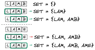
Much like the bloom filter this has the property of no false negatives (i.e. any n-gram not in the set must be from a misspelled word) with the potential for false positives (i.e. can construct a word from the n-grams set that is not a valid word from the original dictionary). 

For the 6.6M dictionary, the following table indicates the space necessary to encode all of the n-grams of a particular size. 

NSize
21,766
333,892
4330,872
51,459,024

To keep within the size constrains of the problem I could only use n-grams of size 2 or 3. I wanted the larger since this was for validation and I felt there would be higher false positive rate using the shorter n-gram size (although, to be fair, I did not measure this).

Building Metadata into the Executable

As I wanted an all-in-one solution, I serialized both the bloom filter and n-gram set to disk as a separate process before building the executable. 

I used a std::bitset for the bloom filter and made sure to set the size to something divisible by 8 so it was possible to serialize without accounting for padded bits. For the n-gram set I ended up using std::set< std::string > so serialization was just a matter of writing the 3-byte sequences out to file. The order in the set didn't matter so I could simply dump the values contiguously given I knew the n-gram size.

With both data sets serialized to disk I used the linker to generate object files out of the binary data so I could link them when building the final executable.

$ ld -r -b binary -o ngram_data.o ngram.bin

$ nm ngram_data.o 
0000000000008464 D _binary_ngram_bin_end
0000000000008464 A _binary_ngram_bin_size
0000000000000000 D _binary_ngram_bin_start


Limitations

Capitalization: To achieve some of the size results I had to make some concessions. For example, all string operations (hashing and n-gram) is performed on lower case strings. This completely removes any capitalization support in this application (a necessary feature for any serious spell checker). 

Speed: Because of the way the dictionary is packed, there is a large upfront cost (relative to the check itself) to load the information into usable data structures before a single word can be checked. I would have liked to have had something that could be searched directly from memory but opted for a more simplistic serialization approach instead.

Results

I computed the full dictionary (6.6M) for n-grams of size 3, hashed each of the 654K words for the bloom filter, and serialized and linked each of those into an executable that came in at 243K. 

In the worst test case (replacing 50% of the dictionary words with invalid words) the f-score was about 0.86 without using n-grams and closer to 0.88 with n-gram validation.
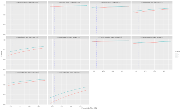

Looking back at the expected false positive rate of the bloom filter (roughly 1 in 3) this is the expected output. With a 654K input, 50% of which are replaced with invalid words, we would expect somewhere around 115K false positives which is consistent with an f-score near 0.85.

Adding in the n-gram effectively helps lower the probability of a false positive from 1 in 3 to just over 1 in 4. There is plenty of room here for optimizations such as fine-tuning the bloom filter to be closer to the size limit, pruning the n-gram list to the most frequent values to reduce size, and so on, but this was a decent start to thinking about the problem.

Wednesday, January 25, 2012

Return on Investment

About a year ago, a friend and I were discussing the evolution of learning new tools while working under time constraints. He claimed that, regardless of the pressure, it is almost always better to sacrifice the upfront time in learning a new tool than to stay in your comfort zone to construct the illusion of progress. By illusion he simply meant that early stage progress is shadowed by the long-term effect of having to maintain and update a homegrown solution.

He used the following illustration to convey his point:


The effect is that if you choose to develop your own tools you satisfy the immediate gratification of results but the final solution is more likely to end up as a house of cards.

I had forgotten about this conversation until recently. The program I am currently working on had me in line to provide relevant results in a shortened amount of time. I am working with the llvm compiler infrastructure and it's unique assembly language. Part of what I needed to do is understand, at a high level, the contents of an llvm assembly file. My natural reaction to this was to implement some minimal parser in Ruby to get to a working set of results quickly. Things went well until I wanted to make a decent tool for broader use within the team: I was starting to spend more time on developing the Ruby code than making headway on my tasks. Not only did I dig myself a grave in that respect but since I was quick to satisyfy the initial demand for results I set an expectation that the work was less complicated than it truly is (and will continue to be). I was building a house of cards.

I ended up scrapping the Ruby implementation and I'm now happily coming up to speed on how to manage llvm code with, well, llvm tools. This is not without effect from the leads of the program, of course. Live and learn, I suppose.

Thursday, August 4, 2011

Hotness

We have an internal image that floated around work several years ago that details network utilization of TCP over a wide variety of configurations. It is a heatmap created in matlab that is just sweet, sweet eye candy. We actually hung it on the outside of a cube for a short while and people couldn't help but stop and look at it.

It is entirely dysfunctional, mind you. The designer tried to combine eight parameters - with all variations - into a individual 2D plot (3D if you consider color a dimension). It was definitely an internal tool - there were only two or three of us who could decipher the layout enough to say anything about the data. That was fine by us; we basically made up the entire population of people who cared.

Fast forward a few years. I'm currently working on a technical report that could use the data we used to create that plot and, as luck would have it, I'm also the only one from the original group still at the company. In order to be able to include this data in the report there needs to occur a certain amount of reformatting - first my brain, then that plot. I wasn't the original designer and, although I have access to the code, I don't know matlab so I'm pretty much stuck. I decided to rework the data in R.

The thing about that original plot was that it had a certain je ne sais quoi: it made you look. I wanted to keep that so I immediately investigated heatmap functionality available in R.

Really? Ouch. Not much available there. I came up with two resources that were helpful: A Wikipedia entry about a Mandelbrot set animation in R; A stackoverflow answer that mentioned rasterImage in a comment. The first site lead me to the color set used in our original plot and the second gave me the pointer I needed to get the job done. I'll leave what follows as a reminder for myself and a helpful nudge for those who face a similar problem in the future.

hmap.example <- function () {

    code <- c("colfun <- colorRampPalette(c(...))",
        "my.colors <- colfun(10000)","xs <- 1:100",
        "X  <- outer(xs,rev(xs))",
        "C1 <- matrix(my.colors[X],100,100)", "X  <- outer(xs,xs)",
        "C2 <- matrix(my.colors[X],100,100)", "X  <- outer(rev(xs),xs)",
        "C3 <- matrix(my.colors[X],100,100)",
        "plot(c(-100,100),c(-100,100),type='n')",
        "rasterImage(C1,1,1,100,100)",
        "rasterImage(C2,-100,1,1,100)", "rasterImage(C3,-100,-100,1,1)",
        "abline(v=0,col='black',lwd=5)", "abline(h=0,col='black',lwd=5)")

    colfun <- colorRampPalette(c("#00007F", "blue", "#007FFF", "cyan",
                    "#7FFF7F", "yellow", "#FF7F00", "red", "#7F0000"))

    my.colors <- colfun(10000)
    xs <- 1:100
    X  <- outer(xs,rev(xs))
    C1 <- matrix(my.colors[X],100,100)
    X  <- outer(xs,xs)
    C2 <- matrix(my.colors[X],100,100)
    X  <- outer(rev(xs),xs)
    C3 <- matrix(my.colors[X],100,100)
    plot(c(-100,100),c(-100,100),type='n',axes=FALSE,xlab='',ylab='')
    rasterImage(C1,1,1,100,100)
    rasterImage(C2,-100,1,1,100)
    rasterImage(C3,-100,-100,1,1)
    abline(v=0,col='black',lwd=5)
    abline(h=0,col='black',lwd=5)
    text(1,1:length(code)*-6,labels=code,cex=0.8,pos=4,family="mono")
}

And the result:

Wednesday, April 13, 2011

Work Ethic

I do something every day at work, something I've done since my first day; I keep details about all things related to hours worked. Mostly this stems from having to manage working 3 or more programs while still billing appropriately for each accurate to the one-half hour. I'll admit that I've also got a slight tendency toward obsessive compulsiveness for some things.

In either case, I decided to take a look back over the past three years to see how my behavior has changed as I've become more comfortable with my surroundings and settled into a personal groove. I should mention first that I work in a very relaxed environment: jeans and t-shirt, flex hours, 24-hour access to premises and so on. This is reflected in the type of patterns that emerge here. Certainly, if I worked at a typical 9-to-5 this exercise would be moot.

Here is what the overall picture looks like[1]:


The blue points represent the times I arrive at work and the red indicates when I leave. You can see a clear pattern - especially in the start times - that is moving away from that 8:30am time. I split the start times into two groups and added a linear fit[2] to bring this out. It follows from this that there should be some split at the top but as each day is not exactly 8 hours the relationship is obviously not 1:1.

Why do the sets diverge then? It made me chuckle when I saw it because I deal with the problem every day and tire of it the more I do. See, I've got a 1-hour commute in each direction. I'm also forced to travel a particularly busy stretch of highway headed into Philadelphia to get to work. When I first started the job I was eager to impress and dealt with traffic to do so. As I've established myself I've decided to either get in early enough to avoid any traffic or wait until it is all passed before heading out. Again, not really possible in the 9-to-5 setting. I don't see actually following the projection lines; the three years have been enough for me to gauge just when to leave. The pattern has probably plateaued by now.

Since I couldn't decipher it from the above image, I also wanted to known what my average output was for the company (and if it had changed as much as my commuting habits). Here is the result: total hours worked for the same time frame shown above.

Takeaway is that I put in, on average, 9 solid hours a day. More obvious is that there is no telling how I'm going to do that over any given period. My first impression was that the hours would be high on Monday decreasing slowly to Friday where the average would be lowest (I like half-day Fridays). There was no such trend, however. In fact, the only day that had any significant difference from the others was Wednesday. I pick my daughter up from school on Wednesday so regardless of what time I get in I leave between 2:30 and 3:30. This ultimately drives down the number of hours I work on Wednesdays over time.

Nothing particularly groundbreaking. While my opinion of the work I do has fluctuated over time I can see no evidence of that in my behavior (from this data, anyway). The traffic thing was a neat find but I was disappointed to not have had more interesting trends in the distribution of hours over the week.

Still, I got to have some fun playing with R and a bit of data.


[1] In all the data presented here I've removed extreme outliers such as a stint I had working 10:00pm to 4:00am. I intended to explore my general behavior so I took some liberties with the data used in doing so.

[2] I failed Prob/Stat the first time through. Literally. I believe there is some underlying assumption about normal distribution when fitting a line which possibly makes this inaccurate as the distribution of each set of points is slightly skewed.